WHAT IS HISTOGRAMMAR

Histogrammar is a free software designed with the idea of being able to represent the most possible detailed image's histogram.

Any 16-bit image has a total of 65536 available levels on each channel; however Photoshop and most tools represent this histogram summarized typically in just 256 possible values. This means that under each of the vertical lines of that PS histogram plot there are as many as 256 different real levels present in the image.

This kind of representation will suffice in most cases, but if we want to perform a deeper analysis we need to use a more detailed image histogram.

Below there is an example of a real histogram represented in the usual range where levels for each channel are restricted to a range of 256 possible values, and what we would obtain if we start to zoom a specific area of this plot thanks to a 16-bit histogram.


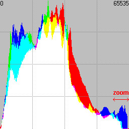
Fig. 1 Classic histogram summarized in 256 levels.


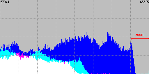
Fig. 2 Zoomed view (16x) of the highlights area.


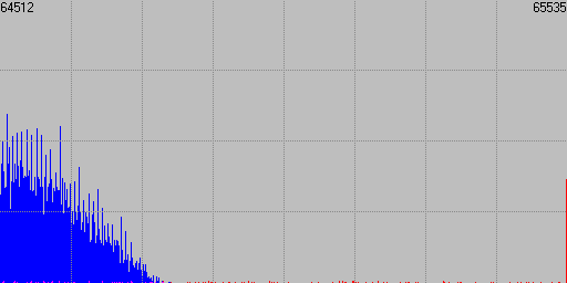
Fig. 3 Zoomed view (128x) of the right end of the highlights area.

The expanded views allow for instance fo find out that there are some few levels in the red channel than blew in the capture, and this could not be detected in the summarized version.

In addition to this Histogrammar allows for a logarithmic scale histogram representation, being this very useful in the analysis of the effective captured dynamic range of the scene along an f-stops axis.

It also provides the ability to plot RAW histograms when the RAW data have been extracted using the appropiate DCRAW commands that we will study.

OPEN AN IMAGE FILE

The first thing to do in Histogrammar to calculate an image's histogram is to open it with the button with a row of dots. Histogrammar's supported formats are in principle TIFF (both 8 and 16-bit), JPEG and BMP.

The usual reason to use this kind of tool is to analyse 16-bit TIFF image files; however it is totally possible to opern 8-bit files as indicated. In any case the histogram will always be represented in terms of a 16-bit image, so we should not surprise when opening an 8-bit image and seeing that all levels appear separated by empty gaps of 255 holes in the histogram. To have a cleaner representation of this type of histograms is not a problem thanks to the X-axis scaling options that we will discuss later.

Histogrammar makes use of the 16-bit graphic library designed by Pierre E. Gougelet, which can handle a large list of graphic formats including some RAW formats from the main camera vendors. In this way, and although success is not guaranteed, we can try to open image formats different to those already exposed just by typing in the open dialog box the required file extension (*.cr2, *.nef, *.gif, *.*,...), what will show all files that did not appear the first time.

In the case of RAW files the library itself will perform a basic RAW development which must be considered with caution as we actually don't know anything about the used parameters. These could be different to those we use in our regular RAW developer, so the result could differ noticeably from expected.


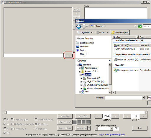
Fig. 4 Open an image file in Histogrammar.

Once the image has been selected in a few seconds Histogrammar will display the histogram and all options that were not enabled until now will become active.

LINEAR vs LOGARITHMIC MODE

As commented, Histogrammar can represent the histogram both in linear (the usual we are accustomed to see in almost all graphic applications) and logarithmic mode.

To switch between these two modes we must press the 'Linear → Log' or 'Log → Linear' option according to the present mode.


WHAT IS A LOGARITHMIC HISTOGRAM

A logarithmic histogram is the one that displays a series of vertical and equally spaced divisions corresponding to each of the different f-stops of the analysed image. The X axis of a logarithmic histogram does not display a linear range of levels but logarithmic, where each of the divisions we mentioned represents a level twice as high as the preceeding one and half of the next division.

Following next there is the correspondence between the linear levels from the previous histogram and its logarithmic scale version. We can see how the whole second half of the linear histogram corresponds only to the highest f-stop of the logarithmic histogram, the next quater corresponds to the second f-stop, and so forth.


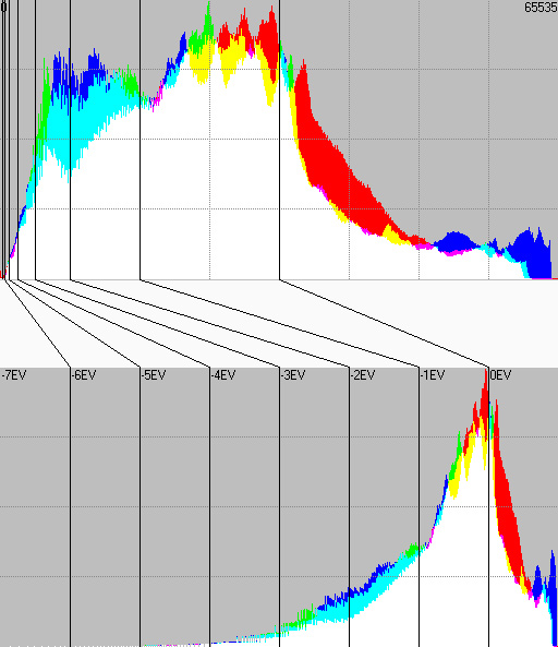
Fig. 5 Correspondence of levels between linear (up) and logarithmic (down) histograms.

In a logarithmic histogram, the 0 level has no place so all black pixels on each channel are excluded from the plot. Strictly speaking they would correspond to the minus infinite f-stop (if you don't see this clear just try to calculate the logarithm of zero).

Also blown pixels are discarded, as although they concentrate in the maximum (level 65535 on a 16-bit range, level 255 on an 8-bit range), they do it simply because there are no higher levels where values could be codified, having reached the sensor saturation. In terms of the luminosity of the real scene these blown pixels would belong to f-stops above the maximum the sensor was able to capture with the exposure parameters used for the shot.

A total of 16 f-stops are calculated (in the example above only the upper 8 were displayed for simplicity), as this is the maximum number of f-stops which can be codified with 16 bits. It is important however to interpret with care the meaning of the lowest f-stops, as our camera in general will not be able to capture a dynamic range beyond the 8 upper f-stops.

That means that any level falling into the lowest f-stops will be there, rather than for being this its real luminance position in the zone system of the scene, because of the presence of noise in the shadows that finally propiciated the level being codified in that place, instead of appearing as pure black.

It makes sense however to calculate so many f-stops as for the case of images obtained by blending different shots with different exposure values, we will be able to exceed the physical limits of the dynamic range of the sensor. In this way we will be able to correctly capture more diaphragms than those we can achieve in a single shot.


WHEN A LOGARITHMIC HISTOGRAM MAKES SENSE

The main advantage of a logarithmic histogram is to stablish a straight connection between the light distribution calculated in f-stops over that histogram, and the real light distribution present in the captured scene. To make that matching happen there is only one condition: to have an histogram calculated over a linear format image.

If this premise is true, for sensor linearity we can be sure that the f-stops distribution showed by Histogrammar will correspond precisely to the luminous information found in each diaphragm of the real scene at shooting time.

Commercial RAW developers do not allow to develop images in linear format. To be able to do that we can just simply use the free RAW developer DCRAW, which is by default a linear developer.

We can use Histogrammar to calculate the histogram in logarithmic mode from a non linear format image (i.e. the kind of image format we are used to handle, with a gamma correction curve applied), but the result will not make much sense as it will not reflect the f-stops distribution of the scene.

We can also calculate the linear mode histogram from a linear format image, but we should be aware to correctly interpret the result as in a linear image levels are severely concentrated to the shadows.


For the rest of the tutorial I made use of the data from the following scene, deliberately chosen for having a high contrast:


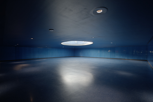
Fig. 6 Scene analysed using Histogrammar.

With a linear format developing of that image we can obtain the following logarithmic mode histogram, which will thus show the real light distribution of the place:


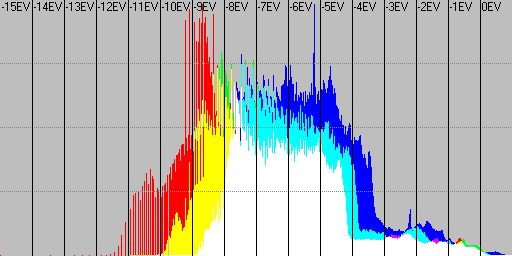
Fig. 7 Logarithmic histogram of linear image (show the real dynamic range of the scene).

So as the linear mode histogram, knowing in this case that most of the information will locate in the shadows due to the absence of gamma correction.


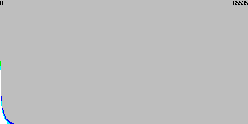
Fig. 8 Linear histogram of linear image.

Linear images as this one display very dark if the visualization tool does not take into account that there is no gamma correction applied. This is not a problem at all when calculating the histogram. On the contrary, the information remains unaltered and its linear condition is what makes the result of the logarithmic histogram perfectly match the real light distribution of the captured scene.

Looking at the logaritmic histogram we can check that the dynamic range of the captured scene was nearly 13 f-stops of real dynamic range, each vertical division corresponding to one diaphragm.

You may wonder how is that possible if the Canon 350D can hardly capture 8 f-stops of dynamic range in one single shot. The answer is that the displayed image was made by blending 3 different shots separated 3 f-stops using the technique commented in Zero noise photography. This is the kind of images that make 16 f-stops logarithmic plots make sense as was already commented.

If we apply the usual gamma corrected developing we would obtain a classical linear mode histogram we are used to, because of the expansion of shades towards the lights according to the correction applied:


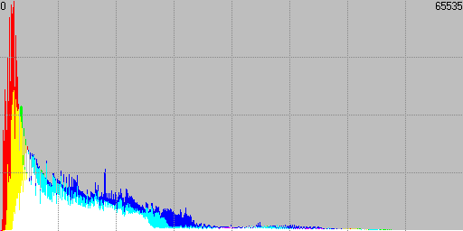
Fig. 9 Linear histogram of gamma corrected image.


MOTIVATION FOR A LOGARITHMIC HISTOGRAM

The main motivation to introduce a logarithmic mode in Histogrammar was that surprisingly, there is no other existing tool performing this. And I consider it very interesting for being a 100% photographic concept.

Even those presumably logarithmic histograms displayed in our cameras, with vertical divisions that make you think of f-stops, are not really logarithmic. To check this it is enough to make a test altering exposure in one f-stop steps and checking that the histogram does not move forward/backwards in a constant amount in each change. We can also check how black areas of the histogram concentrate in the origin of the X axis, which is a conceptual mistake in a strictly logarithmic representation as we commented before.

VISUALIZATION CONTROLS

Histogrammar has a series of visualization controls to set up the graphic output representation to our needs. We will divide them in three blocks: the slide bar, the display options and the zoom levels: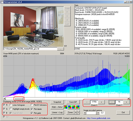


Fig. 10 Visualization controls: slide bar, display options and zoom levels.


SLIDE BAR

We can move along the whole histogram making use of it. At any time, above the histogram plot we will see the maximum value represented on the Y axis of the present visualization, so as the sector currently displayed and the levels or f-stops to which it corresponds according to the active mode.

The relative position of the slide bar will give us an idea of the area of the histogram displayed now, and its thickness represents the portion of the total histogram visible range.


DISPLAY OPTIONS

• 'R, G, B' selects to display or hide any combination of the RGB channels.


• 'Lines histogram' allows to represent a bar or linear histogram, being the last one only recommended when dealing with continuos histogram plot without abrupt peaks and holes.
• 'Highlight empty levels' will mark in a different background colour those levels completely empty simultaneously in the three channels which is very useful to quickly locate histogram nulls. With respect to this, I have designed Histogrammar so that, independently of the Y axis zoom applied, it will always show at least one pixel on all those non empty levels. Therefore any level with no pixel displayed at all will be certainly empty independently of the Y axis zoom selected.
• 'Gamma 1.0' applies a gamma correction for linear images so that they don't display so dark. It does not affect to the internal image data nor the histogram, only to Histogrammar's preview.
• 'Plot EV divisions' will draw vertical lines indicating where each f-stop begins and ends, both in linear or in logarithmic mode.
• 'Plot labels' automatically introduces a numerical label indicating the maximum and minimum levels currently displayed on a linear mode histogram, and f-stop numbers in the case of a logarithmic histogram plot.

ZOOM LEVELS

Special attention deserve the zoom controls both in the X and Y axis:

• 'Zoom X is actually a zoom OUT control: in the beginning the histogram is shown with the maximum degree of detail and by pressing several times the '-' control we will zoom it out so that a larger portion of the total histogram is displayed. In this way the display will be summarized by a factor of two at every press going from 65536 levels to 32768 levels, then 16384 levels,... up to a miminum of 256 levels which represents the typical Photoshop concentrated histogram. Tha data of the extended histogram remain intact so we can press '+' at any time to increse the degree of detail in the visualization.
• 'Zoom Y' on the contrary is a zoom IN control: at first the histogram displays scaled in the Y axis so that the highest value represented corresponds to the absolute histogram maximum. This will probably make unrecognisable those parts of the histgroam containing less pixels where by pressing down the '+' control we will expand the level of zoom over these parts and visualize the content of the lowest amplitued areas of the histogram.

Just to comment that the slide bar, both zoom controls, so as the drawing of the f-stops limits and the labelling of the graphics can be set independently for the linear and logarithmic mode. So when we switch the display mode the program will bring back the region of the histogram displayed, the level of zoom in the X and Y axis that had been set for that mode, so as the drawing of the f-stops borders and their labels.

STATISTICS ABOUT THE ANALYSED IMAGE

At the same time as each pixel's levels are analysed to build the histograms, some statistical analyse is done about the information contained in the image file that is displayed in the status windows once calculations end.

Taking the sample image the information provided is as follows:

   Total pixels: 8038836 (3474x2314 image)
   Black levels: {165;0;13} -> {0%;0%;0%}
   Burnt levels: {696;501;344} -> {0%;0%;0%}
   Histogram maximum: 39736 pixels in level R=82

   Filled levels:
     R: 41447 (63,2% of available)
     G: 37163 (56,7% of available)
     B: 47462 (72,4% of available)
   Dynamic range:
     RGB: 65536 (100% of available), range [0..65535]
     R: 65536 (100% of available), range [0..65535]
     G: 65519 (100% of available), range [17..65535]
     B: 65536 (100% of available), range [0..65535]
   Tonal quality:
     R: 63,2% levels, 134,3% gap std dev, 857,5% ampl std dev
     G: 56,7% levels, 162% gap std dev, 621,1% ampl std dev
     B: 72,4% levels, 144,8% gap std dev, 520,8% ampl std dev

being these the different sections:

• Number of total pixels and size of the image
• Number of pure black (zero value) levels per channel
• Number of blown (saturated) levels per channel
• Absolute maximum of the histogram (pixels, level and channel)
• Number of levels containing some information per channel
• Dynamic range in linear levels per channel
• Tone quality: levels, uniformity of gaps between levels and amplitudes

The last item could require some explanation. Tonal richness is mainly measured by the number of different levels with information, but two other parameters play a role on it that are the regularity in which those non empty levels spread along the histogram's X axis, and the uniformity of the values that the registered levels reach in the histogram's Y axis.

The 'gap std dev' and 'ampl std dev' parameters are measuring this, representing in % the standard deviation relative to the mean separation between filled levels in the histogram's X axis (gap), and the same for the amplitude distribution of the histogram (ampl). Ideally both % values should be as low as possible, 0% in an completely regular distribution of levels both in the X and Y axis of the histogram.

However we must say that these are purely numerical figures that should never condition the best subjective possible result for our image, so they are simply orientative.

When the analysed image is 8-bit, although the histogram plot is represented on a 16-bit basis, the statistical calculated values take as a reference the 8-bit image. So a JPEG file acoounting 200 different non empty levels in the histogram will be qualified with a 200/256=78% filled levels ratio.

GRAPHIC SNAPSHOT OF THE HISTOGRAM

At any time the 'Snapshot' option can be used to dump into the Clipboard a copy of the plot currently being displayed that could then be pasted on any other graphic application.

With the 'Save GIF' option the dump will be performed to an output GIF file using the same saving path as the one from the analysed image. The name of the output file will be indicated on screen and will include the name of the image file.

In general the output image will be 768 pixels wide, except on those cases in which we had set a level of zoom for the X axis so that the histogram becomes smaller than the total available width. So also 512 and 256 pixel graphics are also possible depending on the level of zoom.

REPRESENTATION OF THE IMAGE IN THE ZONE SYSTEM

Taking advantage of the capabilities of Histogrammar to plot logarithmic histograms, I have added a new feature into it which is conceptually very related to photography and will delight anyone interested in the Zone System. It is the possibility of representing in 1 f-stop steps the different luminous areas of the image.

With the 'Zones' options four GIF files of the same size of the image under study will be generated, indicating in a greyscale to which f-stop belongs each of their pixels. Each of the three first files correspond to the RGB channels and the fourth displays the luminosity distribution.

With the 'A/D' control we can choose the type of plot:

• 'A' will display the Ansel Adams' zone system, consisting in 11 light zones from which the upper one is considered as pure white without any detail, and the lower one is black pure also without detail. So the 9 medium zones are the ones containing the information of the scene, where zone V will be middle gray.
• 'D' will plot the zone system corresponding to a 16-bit digital image, where we can differentiate more f-stops with detail than those considered by Ansel Adams up to a total of 16. Burnt pixels will appear in red color and pure black pixels in blue colour. The luminosity will be considered burnt for a pixel only if the three channels are burnt at the same time, and the same will apply to the zero luminosity pixels.

Both representations are completely coherent, simply part of what in the Ansel Adams reprsentation is considered as pure black where no information can be ontained, in the digital 16-bit zone system corresponds to the lower 7 f-stops where we can still find information. To do that today we need to use some dynamic range expansion technique as multiexposure, but it is totally possible to achieve it as can be seen in the sample image. Ansel Adams could not imagine that scenes with such a huge amount of f-stops plenty of information could be captured!.

I have to say however that this is an interpretation of Ansel Adams' zone system model but applied to the scene under capture, while he focused in the printed copy. So it is not strictly the real zone distribution he was talking about. I consider however that in the digital era, taking into account that we can do a very precise control of the luminosity levels on post process, it is much more interesting the concept of dynamic range of the scene, one of the main weak points of today's digital sensors.

We must say however that the Ansel Adams' zone system was oriented to the printed copy, which is where actually makes sense to talk about zones and not in the scene. The matching between f-stops in the scene and zones of zone system only happens in those situations that he used to call normal contrast, which are precisely the ones in which the photographer will want to achieve this one to one relation.

The auxiliar control 'Y/N' allows to choose if on the right side of every generated GIF file we want to display a greyscale bar indicating the different grey tones corresponding to each f-stop, that in the case of the Ansel Adams' mode will be labelled in the same way as he did.

The same as when we talked about the logarithmic histogram, to make this calculation make sense and obtain the real distribution of luminosity in the captured scene we must necessarily start from a linear format image file.

By making use of these feature for the sample image used in the tutorial we obtain the following distributions:


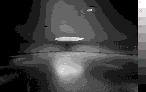
Fig. 11 Ansel Adams' zone system of the scene.


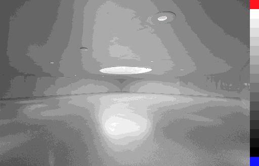
Fig. 12 16-bit zone system of the scene.

Noisy images can show certain grain in the transitions of the lower f-stops because of noise. Also there can be some grain in images where pixels with considerably different luminosity values share the same area.

This last is the case of the sample image, which is practically free of noise but has a very grainy texture on the floor with important luminosity changes, hence the grain appearing in the border limits between diaphragms. On the contrary this phenomenon does not show on the walls or on the ceiling.

In order to prevent this granulation to distract out attention from the zone analysis of the image, it is very effective to apply some median blur filter to the image, or a gaussian blur, followed by a posterization process to the same number of grey tones as we are working with.

PHOTOSHOP'S 15-BIT IMAGES

In a usual edition workflow today the image will eventually fall into Photoshop. PS, for reasons that are not very clear from Adobe, automatically "steals" from our images the least representative bit so Photoshop actually performs a 15-bit edition.

With this loss half of the total possible tone levels are discarded reducing from 65536 to 32768. In terms of dynamic range, and always talking about linear image files, this means we are losing a whole f-stop from the originally 16 available.

The amount of levels is still more than enough for any kind of post processing without posterization or similar problems for this reason in most cases, but the true is that is not a happy idea to work with half the precision without knowing very well why and specially without a warn.

With Histogrammar we can check this phenomenon, in fact I comment this here in case you get a surprise when analysing the histogram of one of your favourite pictures and you realise that where you expected to find a continuous histogram you actually find a comb shape histogram with levels alternatively empty.

Taking as an example the linear image used in this tutorial, we will compare the original histogram at a maximum degree of detail with the one we get after opening and saving it back from PS, both in 16-bit TIFF format:


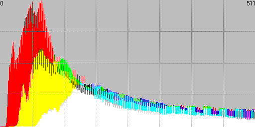
Fig. 13 Original linear histogram.


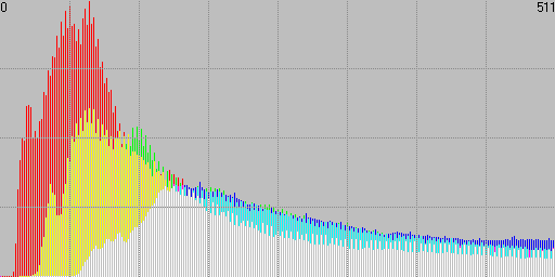
Fig. 14 Linear histogram after open and save action in PS.

Looking at this maybe we should put the sentence "TIFF is a lossless format" under revision, and add a disclaimer "...unless you go to Photoshop!".

Strictly speaking Photoshop works in 15 bits plus one level. It uses a total number of 32769 levels: the even values from 0 to 32768, and the odd ones from 32769 to 65535. In practice this is equivalent to a 15-bit encoding.


~~~

If this content has been useful to you, please consider making a contribution to support this site. Keeping it means an important effort, so as considerable storage space and bandwidth in the server. It is a simple and totally secure operation.