INTRODUCTION

The idea is to develop a simple method compatible with the regular shooting technique, to completely eliminate noise from our shots even in the deepest shadows.

In this way we will recover all textures that noise made unusable and at the same time we will expand the effective dynamic range of our camera in the low light end.

We will make use of two concepts:


DYNAMIC RANGE

Digital cameras have a dynamic range limited basically by noise, and also by the shortage of tone levels available to represent the low f-stops of the image. By experimenting I estimated that the Canon 350D's dynamic range at ISO100 is about 8 f-stops. We all know that even in the lowest ISO number noise appears in the deep shadows making those areas almost unusable, specially when the dynamic range of the scene is high.

On the other hand the number of bits in which RAW data are codified means a physical limit, or we would rather say a mathematical limit, to the dynamic range in an only shot. For the case of the Canon 350D and most DSLR cameras, RAW files are codified into 12-bit samples being limited for this reason to a maximum of 12 f-stops and 4096 linear tone levels.

If we labelled as 0EV the highest f-stop, the distribution of levels in those 12 f-stops would be as follows:

    0EV: 2048 levels, 2048..4095
   -1EV: 1024 levels, 1024..2047
   -2EV: 512 levels, 512..1023
   -3EV: 256 levels, 256..511
   -4EV: 128 levels, 128..255
   -5EV: 64 levels, 64..127
   -6EV: 32 levels, 32..63
   -7EV: 16 levels, 16..31
   -8EV: 8 levels, 8..15
   -9EV: 4 levels, 4..7
   -10EV: 2 levels, 2..3
   -11EV: 1 level, 1

It is clear that even in a theoretical absence of noise, it would be complicated to admit that we are properly registering those lowest f-stops as they are poorly represented in terms of tonal richness. We would be talking in that case of a quantification noise due to excessive digital round errors.


EXPOSE TO THE RIGHT

It is well known the improvement in the signal to noise ratio and tone quality achieved when overexposing a shot and correcting this overexposure in the RAW development stage; what we usually know as right exposure.

It can be demonstrated that for every additional f-stop in exposure, perceived noise in the deep shadows is aproximately halved with respect to what we would obtain without applying that overexposure. So with a +1EV overexposure we will reduce noise to 50%, with +2EV to 25%, and so forth.

There is also an improvement in tonal richness, or we would rather say in tone precision, thanks to the right exposure. This improvement however, and despite of what some specialized bibliography states, for the nature of Bayer interpolation algorithms is not going to be actually noticeable in the quality of results if only moderated overexposures are applied.

"TECHNIQUE OF THE 4 F-STOPS"

By joining those two concepts I have tested what I call the "Technique of the 4 f-stops", consisting in making an additional shot of the same escene in parallel to the one we did in normal conditions, but in this ocasion with a severe overexposure of 4 f-stops (hence the name of the method). The figure was carefully chosen as 4 is right the amount necessary to rescue those lowest 4 f-stops corresponding to the deepest shadows in the scene, eliminating noise from them and restoring all textures with a great tonal richness.

The technique requires the utilisation of a tripod to have a perfect match between both shots, and it may also sound logical in a noise reduction application set our camera in its lowest possible sensitivity (typically ISO100).

We will achieve the overexposure by reducing shutter speed as in the case of opening our camera's diaphragm we would get a different depth of field in each shot that would lead to an unnatural and strange result.

One last point to consider is that the white balance should also be the same in all shots, so it could be convenient to use some of our camera's presets according to the scene particular lighting, avoiding in any case the use of automatic white balance that surely will change somewhat from one shot to the next.

So the steps to be done are:

1. Shoot the scene in a correct exposure according to our usual workflow
2. Repeat the shot now reducing shutter speed by 4 f-stops that will be corrected in the RAW development
3. Blend in some way both images obtaining a free of noise final image

For an even improved result, and if the scene's dynamic range allows to, the correct exposure shot could even be exposed to the right always taking care of not blowing any highlight area as this is the image from which we will eventually obtain the highlights for the final photography.

In the overexposed shot we will not take care of any possible wide areas blown in one or more channels, what is in fact totally expected. As you may guess we will use this shot just to recover the detail in the shadows.

There are other techniques to improve signal to noise ratio such as mean stacking (i.e. average several shots of the same scene), median stacking (eliminate shot noise from images through a more advanced statistical tool that discards the most noisy pixels),... but in digital photography none of them is so powerful as overexposed multiexposure because:

• While mean stacking for instance improves SNR by a factor of N^0.5 being N the number of shots, overexposure blending improves by 2^M being M the number of f-stops apart the second shot was taken. So in case M=4 is chosen, we would reduce noise with just two shots to 1/16 the noise found in the shadows of the original image while we would need as many as N=256 shots to obtain the same noise reduction using simple mean stacking.
• Moreover stacking techniques require a higher precision in the alignment of images since all of them will participate in the final image for every single pixel, so it is easy to loose sharpness when alignment is not perfect. With individual pixel selection in multiexposure blending the loss of sharpness is reduced to a minimum and could happen just in the border areas of the pixels coming from one or the other image.
• In the last place, stacking techniques do not improve tonal richness so even if they can expand dynamic range thanks to noise reduction in the shadows, the resulting image will not be so resistant against posterization as with overexposure blending. If two shots 4 f-stops apart are combined, the density of levels in the shadows is multiplied by a factor of 2⁴=16.

PRACTICAL EXAMPLE

I have written a program to perform with high accuracy and speed the blending process obtaining a final result free of noise and with all textures completely recovered.

For the experiment I chose a high contrast scene which guarantees a strong presence of noise in the shadows even when using the lowest possible sensitivity. With my Canon 350D at ISO100 I did the following shot of the scene in the usual way:



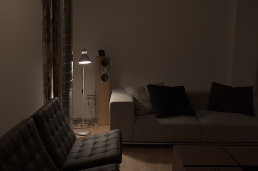
Fig. 1 Original shot with correct exposure to preserve highlight areas.

Now we take a second shot overxposing by 4 f-stops and the result is this:


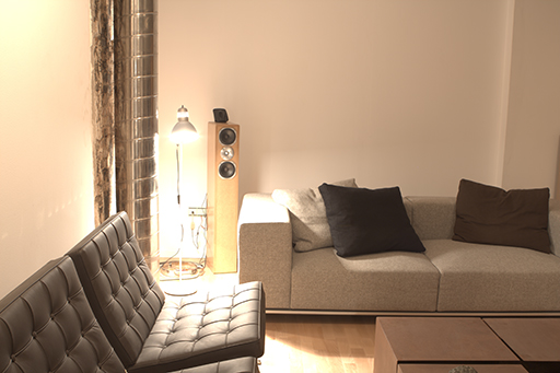
Fig. 2 Shot overexposed by 4 f-stops with respect to the original.

After running the blending algorithm we obtain the following resulting image:


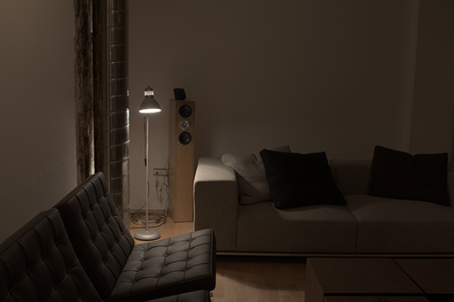
Fig. 3 Image result of blending the original and overexposed shots.

Apparently the final image does not differ in any way from the original: the brightness level was kept and neither scene's contrast nor tones have been altered.

However if we look closely, we will paradoxically see that banding on the background wall is now more visible. These soft bands are due to the 8-bit JPEG conversion and already existed in the original shot, but their transitions were masked thanks to noise. That they have become more apparent is a probe that a clear noise reduction took place, so this is by no means the result of any posterization undesirable effect.

Leaving aside this collateral effect, where is the improvement then? to find out we need to dive into the deepest shadows of the image and analyse them in detail:


16-BIT HISTOGRAMS

Making use of Histogrammar we can calculate the detailed linear histograms of both the original shot and the image resulting of blending it with the overexposed and corrected shot:


Fig. 4 16-bit histogram of the original shot with correct exposure.


Fig. 5 16-bit histogram of resulting image.

The displayed sections correspond to the low region of the histogram, i.e. the deepest shadows of the scene that is where we will be able to notice the highest improvement. It is not necessary to look too closely to realize which of those two histograms provides a better quality.

In the first place in the original histogram the peaks that represent levels captured by the sensor (i.e. non interpolated) are widely separated from each other, suggesting a low tone precission. On the other hand in the resulting image these peaks are so close to each other that almost overlap merging with interpolated levels and producing a soft curve with no comb effect.

It is important to note that the original image presents a strong peak in level 0 for the blue channel. In fact that is the absolute maximum of the whole histogram meaning that in the original shot there exists a large amount of pixels that went totally black at least in that channel. But in the resulting image the histogram fades softly to 0 so it can be concluded that no pixel in the image lost detail for going black.

At last I would like to point that if we look at the blue channel in the second histogram, we will see that in the right end of it the same peaks found on the first histogram start to appear. This is because in this area we are getting far enough from the shadows so that the algorithm started to obtain information from the least exposed shot, i.e. the original one.


NOISE AND TEXTURES IN THE DEEP SHADOWS

An improved histogram can suggest a wider tonal richness and better definition on bright and colour transitions, but if noise were still there in the same way as it appeared in the original image we could not enjoy these advantages. So let us have a look at the perceived improvement in the signal to noise ratio and textures achieved with the contribution of information from the overexposed image.

Several areas have been tested in the dark zones of the image by applying to both images, original and result, the same curve to increase brightness so we are able to measure the improvement. All RAW developments were done using DCRAW with flat parameters, without any kind of sharpening mask, noise reduction or processing of any kind. This is the reason of their dull appearance:


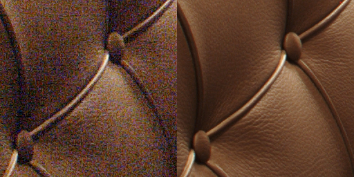
Fig. 6 Comparision between original/result crop 100% middle shadows (chair).


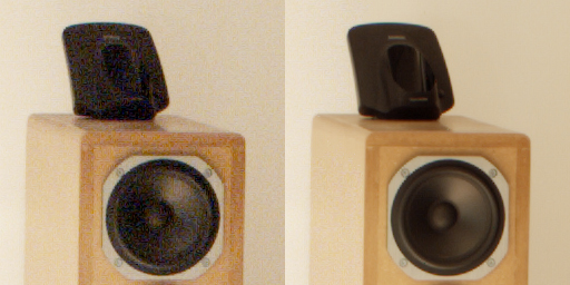
Fig. 7 Comparision between original/result crop 100% deep shadows (loudspeaker).


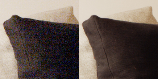
Fig. 8 Comparision between original/result crop 100% very deep shadows (cushion).

As can be apreciated noise reduction and tone quality improvement work together to achieve a higher dynamic range image in the shadows and with a great tonal richness, even in those areas where it is simply impossible to obtain any detail in just one shot.

It is important to be aware that we are analysing really dark areas of the scene. In fact they are so dark that normally we would renounce to get anything from there making them be simply pure black (this is the case of the cushion for instance).


DYNAMIC RANGE HISTOGRAMS

Let us have last a look at the overall logarithmic histogram plots to check how the definition of the lowest f-stops is improved. To do this we will make again use of Histogrammar that allows to calculate logarithmic histograms showing the f-stop distribution of the scene from linear images:


Fig. 9 Logarithmic histogram of the original shot with correct exposure.


Fig. 10 Logarithmic histogram of resulting image.

From the first histogram, we can appreciate that f-stops ranging 0EV to -7EV are acceptably well defined, but from -8EV on available levels are insufficient and variance makes us think that no detail is available in the darkest areas of the image because of noise.

On the other side, the second histogram shows that acceptably well defined levels extend by 4 additional diaphragms as predicted, ranging now f-stops 0EV to -11EV.

We have expanded then the effective captured dynamic range by 4 f-stops, from the original 8 f-stops to the 12 f-stops present in the final image. But differently as in typical HDR tools that apply local microcontrast and tone mapping procedures, the described technique seeks to rescue all possible information providing it in a resulting image with the same overall and local brightness, contrast and tones as the original. It is now a decision of each user to choose the way to process and make use of it in the most convenient way.

~~~
As a conclusion with this method we have turned a modest camera into a virtually free of noise camera. And we did it without leaving aside our daily usual workflow as we just needed to take an additional shot simply adding overexposure.

HOW TO ACHIEVE THE BLENDING OF THE TWO IMAGES

ZERO NOISE PROGRAM

The ideas described until now are not new, the new thing consists of applying them with the goal of a strong noise reduction in mind and in an automatic way, and as a consequence of this obtaining a dynamic range expansion.

I have developed a piece of software to be able to perform automatically all these operations introducing some additional features such as:

• Arbitrary number of shots for better noise, texture and dynamic range enhancement
• Automatic calculation of relative overexposure between the different shots
• Flexible white balance, gamma and exposure controls
• Anti ghosting algorithm to fix effect of moving parts or wrong image alignment
• Local progressive blending algorithm to smooth abrupt transitions in borders
• Floating point operation to maximise tonal richness in the shadows

The program is called Zero Noise and has a tutorial explaining all the details about it.


PHOTOSHOP TUTORIAL

For those not willing to use Zero Noise, there exists a tutorial by Juan Trujillo where it is explained the way to perform the blending of two images with different exposure by making use of Photoshop's layer masks.

His tutorial clearly shows how to carry out the development of the two RAW files so as the setting of a transparency layer mask to take from each shot the desired parts of the scene.

Moreover Juan explains the needed methods to manually implement a powerful, simple and adjustable:

• Progressive blending: to avoid artifacts in the border areas
• Anti ghosting: to eliminate problems with moving parts of the image

You can find it on the author's web site: Yet another method to reduce noise with two exposures. I strongly recommend its reading since what Juan explains in this tutorial is conceptually flawless to make use of all the findings done in this article.

APPLICATIONS AND SOME REAL CASES

APPLICATIONS OF NOISE REDUCTION THROUGH MULTIEXPOSURE

The "Technique of the 4 f-stops" is not general purpose but quite specific. It requires camera stabilization using a tripod and that has the technical limitations of any blending algorithm as is the need of a static scene. If your scene has moving parts (sea waves, objects being moved by wind, smoke, flames,...) some unpleasant effects may appear that will require to be fixed by hand on post process. I plan however to introduce in my program some algorithm improvements to minimise these effects.

Moreover not in all photography fields noise is such a critical factor, and this reduces a bit more those applications for this technique.

However, given its good results I think it can become a regular tool in a workflow with the goal of obtaining the highest possible quality in applications such as:

• Arquitecture and interiorism
• Studio still life
• High contrast landscaping
• Noiseless HDR with Photomatix, Enfuse,...
• Night or poorly lighted photography
• Photography oriented to zone edition
• Slide and film scanning

As we already said this method is compatible with a regular workflow, just requiring and additional shot. If finally we make use of it we will be able to improve the quality of the result, and in any case not making use of it will not be any problem as we would not have left aside our usual way to proceed.


NOISE REDUCTION SAMPLE IMAGES

What is coming next is an example of application in a real work of high contrast interiors photography.

As can be seen in the first two images, the luminosity gap between the indoor and outdoor areas is so wide that with just one shot we are forced to choose: preserve the interior with detail losing those highlights through the windows (picture left), or preserve the windows view losing texture detail in the shadows because of noise (picture right):


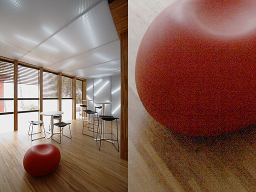
Fig. 11 Result in highlights and shadows in case of taking one only shot.

With the method explained we can have all the information in a unique image file that after a very simple edition produces the following result:


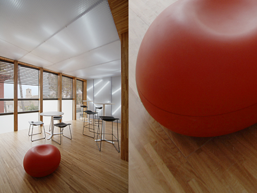
Fig. 12 Result of automated blending of the two previous shots.

More examples from the same session using this method can be found in the tutorial HDR tone mapping. Please notice how well the view through the windows was captured while the dark areas of the images were virtually free of noise.

We can find another example in the Histogrammar tutorial where we analysed an image from a high dynamic range scene containing information along more than 12 f-stops:


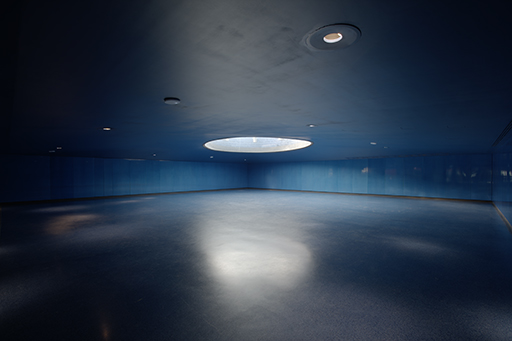
Fig. 13 Free of noise high dynamic range image.

For those interested in seeing in detail what this kind of images look like, the result of blending 3 shots that are 3 f-stops apart can be downloaded from the following link: 11M Memorial. The image is about 13MB size but it is worth to check how powerful noise reduction through multiexposure blending can be.


~~~

If this content has been useful to you, please consider making a contribution to support this site. Keeping it means an important effort, so as considerable storage space and bandwidth in the server. It is a simple and totally secure operation.