INTRODUCTION

We studied in the article Zero noise photography, that by shooting twice over the same scene allowing a generous overexposure on one of the shots, we can achieve a very high reduction in visible noise if the information is blended properly.

This is the basis of Zero Noise, which allows to blend an arbitrary number of RAW files into one TIFF image of minimum noise and maximum sharpness. The improvement in the signal to noise ratio means an expansion in captured dynamic range.

However one of the drawbacks of Zero Noise, and so far of all RAW blending software such as Photomatix or Photoshop HDR, is that they perform the development of the input RAW files making the user loose control over this process.

Present RAW developers, with functionalities to make adjustments over the image so as for other tasks not directly linked to edition such as image classification, play an important role in the user's workflow. It is easy to understand that the photographer does not feel comfortable if he has to carry out the blending of images through an external software that forces him to forget about his usual RAW developer.

This problem would be solved if the blending program outputs another RAW file, that every user could process with his favourite developer or HDR tone mapping software. And this is exactly what Byte Delight has in mind with a new version of Zero Noise that produces an unprocessed RAW output.

To build this virtual RAW we need to make an optimal lossless blending, so that no useful information is lost in the process. Only in that way the resulting file will completely summarize all the information contained in the input files:


Fig. 1 Fusion of information from several RAW files into a unique output virtual RAW.

RAW FUSION PROCESS

Now we will comment the different stages in the fusion process of RAW files into one final virtual RAW:

1. RAW INFORMATION EXTRACTION

To extract all the data contained in the input RAW files we will use DCRAW, that allows to extract 100% raw data with the -D option, or applying with the -d option a linear rescaling from the original native sensor bitdepth up to the 16-bit range.

We will use the -d command that besides converting to 16 bits, corrects the black point when required (typical on Canons), and adjusts the saturation point that for some cameras is a bit lower than the top of their bitscale. Both processes are necessary and mean no information loss.

We could even apply the white balance here, but in this case it is not recommended since it would mean losing information. So the final DCRAW command used is:

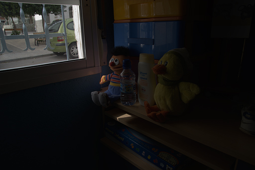
dcraw -v -d -r 1 1 1 1 -4 -T
We will take as an example the fusion of two RAW files obtained with the Canon 350D, applying a difference of 4 stops in exposure. They correspond to the following scene:


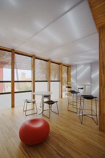
Fig. 2 Scene used as an example for the RAW fusion.

It is a high dynamic range scene impossible to capture in a single shot. In case of preserving the outdoor views, the interior shadows would display excessive noise. And a correct exposure for the indoor area would blow away the information through the windows.

We used an exposure scheme {0EV, +4EV}, where the least exposed shot consists of an exposed to the right capture just before starting to blow the highlights, and the other is an additional shot exposed 4 extra stops.

Even if the raw data themselves do not constitute a viewable image, we can display them in the form of a mosaic to observe the Bayer pattern of the sensor. Focusing on the church area looking through the window we get:


Fig. 3 Crop at 300% of Bayer pattern in one of the original RAW files.

2. OPTIMAL RAW FUSION

RAW FUSION vs TIFF FUSION

Once we have all the needed information to generate the output virtual RAW, we will proceed to blend the images using Zero Noise, which has been adapted to work with RAW data.

Actually the changes needed were few, basically eliminating from the process those steps that do not make sense any more with a RAW output in mind: white balance and output profile selection, so as the RAW interpolation algorithm.

An advantage of working without the white balance is that we can now be more precise in the thresholds to consider valid a certain level in a pixel. In the former TIFF version of Zero Noise, white balance could make us involuntarily more conservative in the evaluation of overexposed channels.

We could also think that blending non interpolated data would allow us to deal separately with the R, G₁, G₂ and B channels, so that any partial saturation in them would not invalidate the values of other channels in adjacent pixels. In that way we could fine tune independent fusion maps for every individual channel.

But it did not work. If the G and R channels for instace get saturated, the B channel yields erroneously high values in adjacent pixels than in case of being considered produce visible exposure gaps. In this situation there is no possible improvement with respect to the fusion maps in the TIFF version of Zero Noise.

This behaviour of the sensor matches the observations done when calculating its response curve in Analogue vs digital photography, where in Fig. 3 it was clear how the B channel showed a small non linearity in the end of the plot, right when the G and B channels got saturated.

We have to check the possibility of storing the final RAW in a non linear way, i.e. with some gamma curve applied. This is already done in the TIFF version of Zero Noise and means more levels in the shadows that could be useful to avoid posterization if they are strongly "lifted". A real example of this improvement can be seen in the article TIFF with more than 16 stops of DR.


RELATIVE EXPOSURE CALCULATION AND FUSION MAP

After the issue with the partial saturation, we improved the algorithm for calculating the relative exposure making it more robust against non linearities produced by such saturations.

For the case of the two RAW files used in the example, the calculated relative exposure was exactly 4 stops, which is not usual since some deviation is common:


Fig. 4 Relative exposure histogram for the two sample RAW files.

The fusion algorithms are those originally from Zero Noise and are oriented to minimise progressive blending, i.e. to obtain most pixels in the final image from only one of the source images so that there is no sharpness loss and noise reduction becomes maximum.

In this particular case we set a progressive blending radius of just 2 pixels, providing the following fusion map (move the mouse over the image to switch to the scene):


Fig. 5 Fusion map used in the example scene.

The most exposed shot (RAW 2) provided 84% of the final output information, corresponding to black areas in the fusion map; and the least exposed shot (RAW 1) provided 16% of the final information, white in the fusion map. The exposure of RAW 2 data was corrected down by 4 stops to match the original exposure of RAW 1.

Despite the considerably fragmented map, the progressive blending set only affected 4.6% of the total pixels being the rest genuine pixels taken from just one of the source images.


16-BIT VIRTUAL RAW AND DYNAMIC RANGE

Comparing the RAW histograms we can see that the real bitdepth of the virtual RAW is 16 bits. This provides many more levels in the low f-stops (shadows) than those the least exposed RAW file has, which is a typical 12-bit histogram.

In that way in the 12th f-stop with respect to saturation (signed as -11EV) the RAW 1 has a unique level, while the final RAW has 16 levels, those obtained from the 8th f-stop of RAW 2 (signed as -7EV).


Fig. 6 RAW histograms of the two captures and the resulting virtual RAW.

The green channel accounts twice as many pixels as the red or blue channels because of the RGGB structure of the Bayer matrix. The two green channels G₁ and G₂ were represented together for simplicity.

Regarding dynamic range, because the Canon 350D can capture acceptably free of noise up to 8 f-stops, the 4 stops overexposure should have allowed us to capture up to 12 f-stops which is the total dynamic range of the scene according to the histogram.

As a previous step to the final conversion to RAW format, we added some text which will prove the artificial origin of the output file.

3. DNG 16-BIT EMBEDDING

Once we have the information resulting from blending in the form of 16-bit integer levels, we will embed it into a standard 16-bit DNG RAW file that will need demosaicing to be displayed.

Not much I can tell about the details of this operation since it has been entirely carried out by Egon, as he already did to generate a synthetic RAW file in RAW. The myth of digital negative.

RAW DEVELOPMENT AND FINAL RESULTS

The goal of this story was that the resulting RAW file could be processed in any RAW developer supporting the DNG format, that is why we will use ACR in all the developments following next.


DEEP SHADOWS AND HIGHLIGHTS

If we compare the virtual RAW with the original ones, we can see RAW 1 is very noisy in the shadows while RAW 2 has completely blown highlights. That means that none of the former two could by itself capture completely the dynamic range of the scene, as we already mentioned.

On the other side, the virtual RAW contains all the information of the other two RAW files so it preserves the highlights, and has free of noise shadows.

Here crops at 50% of the deep shadows and crops at 25% of the highlights are shown, comparing the information in the virtual RAW with the original RAWs:


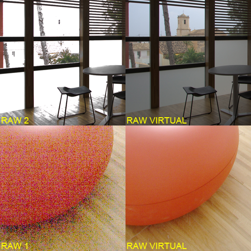
Fig. 7 Deep shadows and highlights comparision original RAWs vs virtual RAW.

With just two shots on a modest Canon 350D, we obtained a virtual RAW file of higher quality in terms of noise and dynamic range than what we would have got from a single shot on any present DSLR, including the last Nikons and the Fuji Super CCD cameras in high dynamic range mode.

At risk of being grandiloquent, we are probably talking about the lowest noise RAW file in the world.


RAW FUSION PARTICULARITIES

One interesting improvement derived from blending in the RAW domain instead of using TIFF files, is that in the leaves of the trees under effect of the wind, that was not taken into consideration when calculating the fusion map, it is not even possible to see any tree movement.

I guess that by blending in the Bayer domain, the interpretation in the development of the moving parts is more natural and progressive than when the RAW files are first separately developed and then blended.

Another advantage when developing the virtual RAW with respect to developing the original RAW files, is that ACR does not eliminate now those border pixels that are rejected in the Canon files.

While RAW 1 and RAW 2 developed in ACR provide 3456x2304 pixels images, the virtual DNG produces a 3474x2314 pixels image, meaning 18 extra pixels in the longer dimension and 10 in the shorter one:


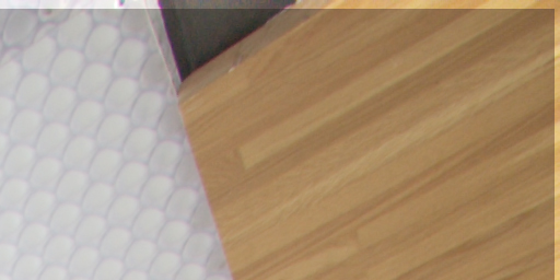
Fig. 8 Extra pixels in the border of the virtual RAW with respect to the original RAW files.

The lens used (Canon 10-22 at 10mm) produced strong chromatic aberrations in the edges against the sky, that obviously travelled from the original RAW files to the virtual RAW. They have no relation with the fusion process.


RAW FUSION vs TONE MAPPING

RAW fusion does not include, nor was intended to, the needed tone mapping to display all the captured dynamic range. They are two well differentiated stages in the process:

1. Zero Noise blends the image producing a RAW (or TIFF) file of maximum quality, but totally unprocessed:
   
RAW FUSION = VIRTUAL CAPTURE

2. Then the user will use his preferred RAW development, HDR tone mapping,... tool to obtain the final image:
   
TONE MAPPING = PROCESSING

If we open the virtual RAW into ACR with all adjustments set to zero, the result is identical to that obtained from the TIFF version of Zero Noise, a totally untouched image:


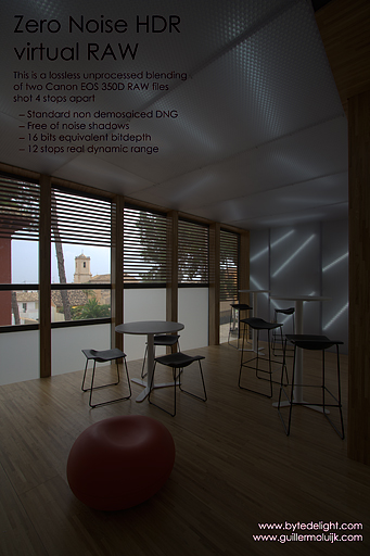
Fig. 9 Result of developing in ACR with all adjustments set to zero.

This initial underexposure is unavoidable in high dynamic range captures when tone mapping has not been applied yet. Without that general underexposure the highlights would be blown, as simple as that. Find here another example of high dynamic range from a Fuji RAF file.

In the HDR tone mapping tutorial there is a proposal to process these underexposed images. However with the new virtual RAW we can now make use of the developer or HDR program to (pre)process it, which was the main goal of the RAW fusion.

So we did adjustments to try to get a finished output HDR image with a natural look in ACR. The key was the tone curve applied to reduce global contrast, brightening the shadows at the same time as the highlights were preserved.

All adjustment parameters are embedded in the DNG file linked below for download, and provide the following result straight from ACR (click on the image to see a 1024px version):


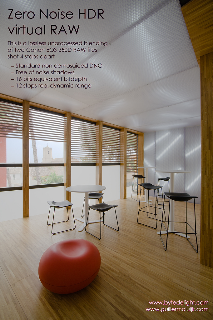
Fig. 10 Result of developing in ACR with tone mapping adjustments.

It can easily be improved with finer postprocessing, specially to avoid the loss of local contrast in the outdoor details. We just wanted to show how the tone mapping of a high dynamic range scene can take place right in the RAW developer, as long as we start from a noiseless RAW file.

DOWNLOAD RAW FILES

For anyone interested in testing, the three RAW files can be downloaded from the following links:

• RAW 1 (7 MB)
• RAW 2 (8.5 MB)
• Virtual RAW (14 MB)

I recommend to download at least the last one. A RAW file of a scene with such a dynamic range, where the shadows can be "lifted" as much as we want without noise appearing is quite impressive.

Making the curve linear it is easy to see the high contrast present in the scene, and how difficult it was to capture it given the limitations of the camera.

CONCLUSION AND APPLICATIONS

We successfully carried out the fusion of several RAW files summarizing all the information contained in them, and obtaining as a result a real 16-bit noise free RAW file that can be processed using any RAW developer supporting the DNG format. As far as I know, this is the first time several RAW files have been fused in the Bayer undemosaiced domain.

As an additional effect to noise reduction we expand the captured dynamic range, which makes the fusion ideal for high contrast scenes (HDR). The fusion is a different process than tone mapping, which is a necessary step in any case.

The resulting file is a high quality source of information, and can be used straight with any program or tone mapping method working from a RAW file. Conceptually the RAW fusion provides captured information, not processed information.

Applications of this technique can be various in fields such as:

• Arquitecture and interiorism
• Studio still life
• High contrast landscaping
• Noiseless HDR with Photomatix, Enfuse,...
• Night or poorly lighted photography
• Photography oriented to zone edition
• Slide and film scanning

Logically any kind of action photography is excluded, since there is no option to use a tripod and have a reasonably static scene.

I think that applying RAW fusion in those high resolution sensors recently appeared on the market (Sony A900 and Canon 5D Mark II), with an accordingly high quality lens, could produce results of the same or even higher quality that with digital backs in a higher price range.

The fusion would compensate the higher per-pixel noise of these sensors due to their high resolution, when compared to lower pixel density cameras. In that way it would be possible to print high dynamic range scenes in sizes up to now out of the reach of a DSLR.

We will try to have ready a usable version of the program, since the method and the implementation of the algorithms have already been solved.


~~~

If this content has been useful to you, please consider making a contribution to support this site. Keeping it means an important effort, so as considerable storage space and bandwidth in the server. It is a simple and totally secure operation.